Introduction

This tutorial introduces the basics of event history analysis (EHA)/survival analysis using the scania dataset from the eha package to study mortality after age 50.

The main idea is to approach the same survival process in two ways. We first estimate survival non-parametrically using Kaplan–Meier (i.e., we do not impose a functional form on the survival process and just examine what the raw data shows). We then restructure the data into person-period format and estimate the age-specific hazard using logistic regression. From those predicted hazards we reconstruct a survival curve and compare it directly with Kaplan–Meier.

After establishing this connection do we add explanatory variables and calculate adjusted survival curves.

Setup

Install the packages if necessary:

Code

install.packages(c(
  "eha",
  "survival",
  "dplyr",
  "tidyr",
  "ggplot2",
  "marginaleffects"
))

Load the packages:

Code

library(eha)
library(survival)
library(dplyr)
library(tidyr)
library(ggplot2)
library(marginaleffects)

Load the Scania data:

Code

data(scania)

head(scania)

    id enter   exit event birthdate    sex parish   ses immigrant
29   1    50 59.242     1  1781.454   male      1 lower        no
66   2    50 53.539     0  1821.350   male      1 lower       yes
70   3    50 62.155     1  1788.936   male      1 lower       yes
83   4    50 65.142     1  1796.219 female      1 lower       yes
100  5    50 51.280     0  1822.713   male      1 lower       yes
132  6    50 70.776     1  1813.547 female      1 lower       yes

Code

summary(scania)

       id             enter         exit           event          birthdate   
 Min.   :   1.0   Min.   :50   Min.   :50.00   Min.   :0.0000   Min.   :1763  
 1st Qu.: 483.5   1st Qu.:50   1st Qu.:55.37   1st Qu.:0.0000   1st Qu.:1786  
 Median : 966.0   Median :50   Median :62.70   Median :1.0000   Median :1808  
 Mean   : 966.0   Mean   :50   Mean   :63.97   Mean   :0.5624   Mean   :1806  
 3rd Qu.:1448.5   3rd Qu.:50   3rd Qu.:72.05   3rd Qu.:1.0000   3rd Qu.:1825  
 Max.   :1931.0   Max.   :50   Max.   :80.00   Max.   :1.0000   Max.   :1845  
     sex      parish      ses       immigrant 
 male  :975   1: 159   upper: 375   no : 759  
 female:956   2: 181   lower:1556   yes:1172  
              3: 180                          
              4: 258                          
              5:1153

The most important variables include:

id: person identifier
enter: age at which observation begins
exit: age at death or censoring
event: whether death occurred at exit
sex: sex
ses: socioeconomic status

In these data, observation starts at age 50.

Suppose a person has:

enter = 50
exit  = 59.24
event = 1

This means that the person is observed from age 50 and dies at age 59.24.

If instead:

enter = 50
exit  = 80
event = 0

the person is observed until age 80 but does not die while under observation. The observation is right-censored.

Survival and the hazard

Two quantities are central to event history analysis.

The survival function

S(t)=P(T>t)

gives the probability of remaining event-free beyond time t.

In our example:

What is the probability that somebody who has reached age 50 survives beyond age 50?

The hazard asks a different question. In discrete time:

h_j = P(\text{death in interval }j \mid \text{alive at the beginning of interval }j).

For example:

Among people who are alive at age 70, what is the probability that they die between ages 70 and 71?

The two quantities are directly connected.

If the hazards in successive intervals are

h_1,h_2,\ldots,h_j,

then survival through interval j is

S_j = \prod_{k=1}^{j}(1-h_k).

This relationship will become important when we estimate the hazard with logistic regression.

Kaplan–Meier survival

We begin with the Kaplan–Meier estimator.

Create a survival object:

Code

surv <- Surv(
  time = scania$enter,
  time2 = scania$exit,
  event = scania$event
)

Because we specify both entry and exit time, this takes the form

Surv(enter, exit, event)

and describes the period during which each person is at risk.

Estimate overall survival:

Code

km <- survfit(
  surv ~ 1,
  data = scania
)

km

Call: survfit(formula = surv ~ 1, data = scania)

        n events median 0.95LCL 0.95UCL
[1,] 1931   1086   69.6    68.9    70.4

Plot the survival curve:

Code

plot(
  km,
  xlab = "Age",
  ylab = "Survival probability",
  main = "Kaplan–Meier survival curve"
)

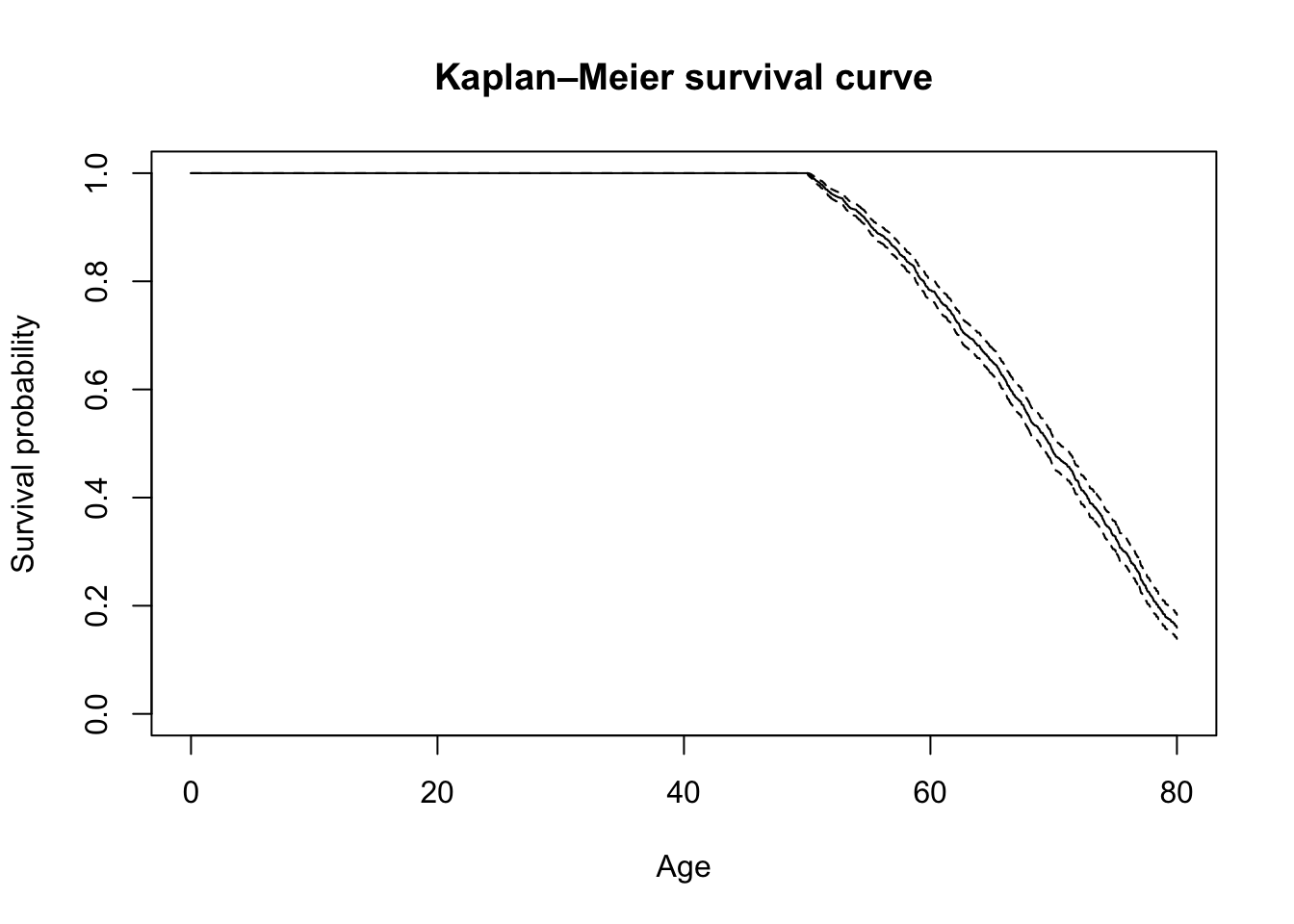
The curve starts at 1 at age 50 and declines as deaths occur.

We can request survival probabilities at selected ages:

Code

summary(
  km,
  times = c(60, 70, 80)
)

Call: survfit(formula = surv ~ 1, data = scania)

 time n.risk n.event survival std.err lower 95% CI upper 95% CI
   60   1129     352    0.783  0.0103        0.763        0.804
   70    578     395    0.483  0.0136        0.457        0.510
   80    146     339    0.159  0.0113        0.139        0.183

For example, the survival probability at age 70 answers:

Among people who survived to age 50, what proportion are estimated to survive to at least age 70?

Kaplan–Meier estimates this directly from the observed survival times. We have not yet specified a regression model.

Person-Period files

To estimate a discrete-time event history model, we restructure the data.

The original data have one row per person.

For discrete-time analysis we instead want one row for every time interval during which a person is at risk.

We will use one-year age intervals.

Someone who dies at age 55.4 will therefore contribute observations approximately like:

id    age    death
1      50      0
1      51      0
1      52      0
1      53      0
1      54      0
1      55      1

The variable death now indicates whether the event occurs during that particular interval.

Thus:

death = 0 means that the person survives the interval.
death = 1 means that the person dies during the interval.

Create the person-period data:

Code

scania_pp <- scania |>
  mutate(
    event = as.integer(event),
    n_intervals = if_else(
      event == 1,
      ceiling(exit) - 50,
      floor(exit) - 50
    )
  ) |>
  filter(n_intervals > 0) |>
  uncount(
    n_intervals,
    .id = "period",
    .remove = FALSE
  ) |>
  mutate(
    age = 49 + period,
    death = as.integer(
      event == 1 &
        period == n_intervals
    )
  )

Inspect the resulting file:

Code

scania_pp |>
  select(id, age, death, sex, ses) |>
  head(20)

   id age death  sex   ses
1   1  50     0 male lower
2   1  51     0 male lower
3   1  52     0 male lower
4   1  53     0 male lower
5   1  54     0 male lower
6   1  55     0 male lower
7   1  56     0 male lower
8   1  57     0 male lower
9   1  58     0 male lower
10  1  59     1 male lower
11  2  50     0 male lower
12  2  51     0 male lower
13  2  52     0 male lower
14  3  50     0 male lower
15  3  51     0 male lower
16  3  52     0 male lower
17  3  53     0 male lower
18  3  54     0 male lower
19  3  55     0 male lower
20  3  56     0 male lower

We can also inspect one person who dies:

Code

example_id <- scania_pp |>
  filter(death == 1) |>
  slice(1) |>
  pull(id)

scania_pp |>
  filter(id == example_id) |>
  select(id, age, death)

   id age death
1   1  50     0
2   1  51     0
3   1  52     0
4   1  53     0
5   1  54     0
6   1  55     0
7   1  56     0
8   1  57     0
9   1  58     0
10  1  59     1

There are multiple observations for this person but only one event, in the final interval.

Discrete-time EHA using logistic regression

We now estimate the same mortality process using logistic regression.

Because each row represents one interval during which a person is at risk, our dependent variable is

P(death_{it}=1).

More precisely, the model estimates

P( \text{death during interval }t \mid \text{alive at the start of interval }t ).

This is the discrete-time hazard.

First model: the baseline hazard only

Before adding explanatory variables such as sex or socioeconomic status, we estimate a model containing only age.

For the first model, it is useful to treat age as categorical:

Code

m0 <- glm(
  death ~ factor(age),
  data = scania_pp,
  family = binomial(link = "logit")
)

summary(m0)


Call:
glm(formula = death ~ factor(age), family = binomial(link = "logit"), 
    data = scania_pp)

Coefficients:
              Estimate Std. Error z value Pr(>|z|)    
(Intercept)   -4.01173    0.17562 -22.843  < 2e-16 ***
factor(age)51  0.19634    0.24028   0.817 0.413875    
factor(age)52 -0.20900    0.27034  -0.773 0.439455    
factor(age)53  0.02659    0.25682   0.104 0.917552    
factor(age)54  0.37212    0.23908   1.557 0.119588    
factor(age)55  0.34960    0.24358   1.435 0.151228    
factor(age)56  0.31006    0.24878   1.246 0.212660    
factor(age)57  0.44690    0.24374   1.834 0.066719 .  
factor(age)58  0.73585    0.23217   3.169 0.001528 ** 
factor(age)59  0.64621    0.23952   2.698 0.006977 ** 
factor(age)60  0.61984    0.24404   2.540 0.011088 *  
factor(age)61  0.73260    0.24114   3.038 0.002381 ** 
factor(age)62  0.91227    0.23483   3.885 0.000102 ***
factor(age)63  0.49083    0.26263   1.869 0.061637 .  
factor(age)64  0.86804    0.24297   3.573 0.000353 ***
factor(age)65  1.06229    0.23643   4.493 7.02e-06 ***
factor(age)66  1.20233    0.23325   5.155 2.54e-07 ***
factor(age)67  1.25633    0.23455   5.356 8.50e-08 ***
factor(age)68  1.15495    0.24377   4.738 2.16e-06 ***
factor(age)69  1.48080    0.23305   6.354 2.10e-10 ***
factor(age)70  0.90007    0.27270   3.301 0.000965 ***
factor(age)71  1.48703    0.24195   6.146 7.94e-10 ***
factor(age)72  1.73214    0.23642   7.326 2.36e-13 ***
factor(age)73  1.51389    0.25429   5.953 2.63e-09 ***
factor(age)74  1.70036    0.25134   6.765 1.33e-11 ***
factor(age)75  1.87335    0.25056   7.477 7.63e-14 ***
factor(age)76  2.10805    0.24714   8.530  < 2e-16 ***
factor(age)77  2.36307    0.24627   9.595  < 2e-16 ***
factor(age)78  2.25964    0.26449   8.543  < 2e-16 ***
factor(age)79  2.16362    0.28490   7.594 3.10e-14 ***
---
Signif. codes:  0 '***' 0.001 '**' 0.01 '*' 0.05 '.' 0.1 ' ' 1

(Dispersion parameter for binomial family taken to be 1)

    Null deviance: 9121.7  on 27177  degrees of freedom
Residual deviance: 8685.2  on 27148  degrees of freedom
AIC: 8745.2

Number of Fisher Scoring iterations: 6

Why use factor(age)?

Because we do not yet want to impose a particular shape on the baseline hazard.

Instead, the model estimates a separate mortality probability for each age interval.

Conceptually, this model is estimating

h_{50}, h_{51}, h_{52}, \ldots

where, for example, h_{70} is the probability of dying between approximately age 70 and 71 among people who are alive at age 70.

Predicted hazards using `marginaleffects`

The coefficients from a logistic regression are expressed as log odds.

Those are usually not the most useful quantities for interpretation.

We can instead use marginaleffects to obtain predicted probabilities.

Code

hazard0 <- predictions(
  m0,
  newdata = datagrid(
    age = sort(unique(scania_pp$age))
  ),
  type = "response"
)

hazard0


 age Estimate Std. Error    z Pr(>|z|)    S   2.5 % 97.5 %
  50   0.0178    0.00307 5.80   <0.001 27.1 0.01177 0.0238
  51   0.0216    0.00346 6.23   <0.001 31.0 0.01478 0.0283
  52   0.0145    0.00293 4.94   <0.001 20.3 0.00873 0.0202
  53   0.0183    0.00336 5.44   <0.001 24.1 0.01167 0.0248
  54   0.0256    0.00404 6.33   <0.001 31.9 0.01766 0.0335
  55   0.0250    0.00412 6.08   <0.001 29.6 0.01696 0.0331
  56   0.0241    0.00414 5.82   <0.001 27.3 0.01597 0.0322
  57   0.0275    0.00452 6.08   <0.001 29.7 0.01866 0.0364
  58   0.0364    0.00533 6.83   <0.001 36.8 0.02597 0.0468
  59   0.0334    0.00526 6.35   <0.001 32.1 0.02309 0.0437
  60   0.0325    0.00534 6.10   <0.001 29.8 0.02209 0.0430
  61   0.0363    0.00578 6.28   <0.001 31.5 0.02497 0.0476
  62   0.0431    0.00643 6.70   <0.001 35.5 0.03052 0.0557
  63   0.0287    0.00545 5.27   <0.001 22.8 0.01805 0.0394
  64   0.0413    0.00665 6.21   <0.001 30.8 0.02830 0.0544
  65   0.0498    0.00749 6.65   <0.001 35.0 0.03509 0.0644
  66   0.0568    0.00823 6.91   <0.001 37.6 0.04070 0.0729
  67   0.0598    0.00874 6.84   <0.001 36.9 0.04265 0.0769
  68   0.0543    0.00869 6.26   <0.001 31.2 0.03731 0.0714
  69   0.0737    0.01046 7.05   <0.001 39.0 0.05322 0.0942
  70   0.0426    0.00851 5.01   <0.001 20.8 0.02594 0.0593
  71   0.0741    0.01142 6.49   <0.001 33.4 0.05175 0.0965
  72   0.0928    0.01333 6.96   <0.001 38.1 0.06670 0.1190
  73   0.0760    0.01292 5.88   <0.001 27.9 0.05069 0.1013
  74   0.0902    0.01475 6.11   <0.001 29.9 0.06127 0.1191
  75   0.1054    0.01685 6.25   <0.001 31.2 0.07239 0.1385
  76   0.1297    0.01963 6.61   <0.001 34.6 0.09122 0.1682
  77   0.1613    0.02336 6.91   <0.001 37.5 0.11551 0.2071
  78   0.1478    0.02491 5.93   <0.001 28.3 0.09896 0.1966
  79   0.1361    0.02638 5.16   <0.001 21.9 0.08440 0.1878

Type: response

The variable estimate now contains the estimated probability of dying during each age interval.

Code

hazard0 |>
  as.data.frame() |>
  select(age, estimate)

   age   estimate
1   50 0.01778017
2   51 0.02155417
3   52 0.01447528
4   53 0.01825047
5   54 0.02559055
6   55 0.02503477
7   56 0.02408759
8   57 0.02752294
9   58 0.03640777
10  59 0.03339041
11  60 0.03254973
12  61 0.03629417
13  62 0.04312939
14  63 0.02872340
15  64 0.04134078
16  65 0.04976303
17  66 0.05681818
18  67 0.05978261
19  68 0.05433186
20  69 0.07371795
21  70 0.04262877
22  71 0.07414449
23  72 0.09282700
24  73 0.07600950
25  74 0.09018568
26  75 0.10542169
27  76 0.12969283
28  77 0.16129032
29  78 0.14778325
30  79 0.13609467

An estimate such as

age      = 59
estimate = 0.033

would mean:

Among people who have survived to age 59, approximately 3.33% are predicted to die during the following age interval.

This is a hazard probability, not a survival probability.

From predicted hazards back to survival

We can now convert the predicted hazards into a survival curve.

Recall:

S_j = \prod_{k=1}^{j}(1-h_k).

Using R, this cumulative product is calculated with cumprod().

Code

surv0 <- hazard0 |>
  as.data.frame() |>
  mutate(age = as.numeric(levels(age))) |>
  arrange(age) |>
  mutate(
    survival = cumprod(1 - estimate),
    age_end = age + 1
  )

Inspect the result:

Code

surv0 |>
  select(
    age,
    estimate,
    age_end,
    survival
  )

   age   estimate age_end  survival
1   50 0.01778017      51 0.9822198
2   51 0.02155417      52 0.9610489
3   52 0.01447528      53 0.9471374
4   53 0.01825047      54 0.9298517
5   54 0.02559055      55 0.9060563
6   55 0.02503477      56 0.8833734
7   56 0.02408759      57 0.8620951
8   57 0.02752294      58 0.8383677
9   58 0.03640777      59 0.8078446
10  59 0.03339041      60 0.7808703
11  60 0.03254973      61 0.7554532
12  61 0.03629417      62 0.7280347
13  62 0.04312939      63 0.6966350
14  63 0.02872340      64 0.6766252
15  64 0.04134078      65 0.6486530
16  65 0.04976303      66 0.6163741
17  66 0.05681818      67 0.5813528
18  67 0.05978261      68 0.5465980
19  68 0.05433186      69 0.5169003
20  69 0.07371795      70 0.4787955
21  70 0.04262877      71 0.4583850
22  71 0.07414449      72 0.4243983
23  72 0.09282700      73 0.3850027
24  73 0.07600950      74 0.3557388
25  74 0.09018568      75 0.3236563
26  75 0.10542169      76 0.2895359
27  76 0.12969283      77 0.2519852
28  77 0.16129032      78 0.2113424
29  78 0.14778325      79 0.1801095
30  79 0.13609467      80 0.1555976

For every interval:

estimate is the probability of dying during the interval.
survival is the probability of surviving all intervals up to its end.

Plot the model-based survival curve:

Code

ggplot(
  surv0,
  aes(
    x = age_end,
    y = survival
  )
) +
  geom_line(linewidth = 1) +
  labs(
    x = "Age",
    y = "Survival probability",
    title = "Survival derived from discrete-time logistic regression"
  ) +
  theme_minimal()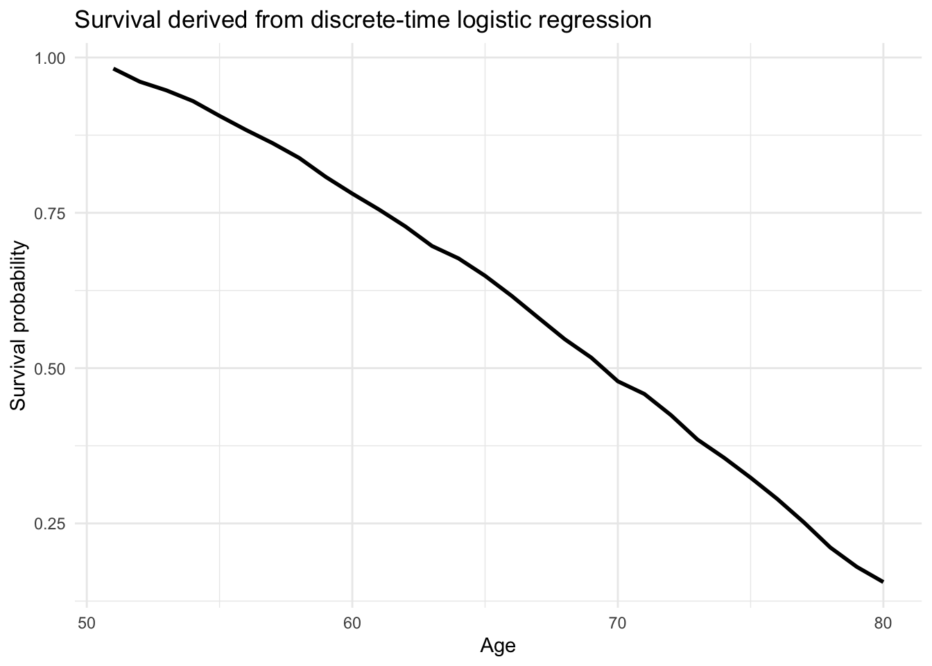

Comparing logistic regression with Kaplan–Meier

We can now compare the two approaches.

First extract the Kaplan–Meier estimates:

Code

km_summary <- summary(km)

km_df <- data.frame(
  age = km_summary$time,
  survival = km_summary$surv
)

Then plot the Kaplan–Meier curve together with the survival curve reconstructed from the discrete-time logistic regression:

Code

ggplot() +
  geom_step(
    data = km_df,
    aes(
      x = age,
      y = survival
    ),
    linewidth = 0.9
  ) +
  geom_line(
    data = surv0,
    aes(
      x = age_end,
      y = survival
    ),
    linewidth = 1,
    color = 'red',
    alpha = 0.7
  ) +
  labs(
    x = "Age",
    y = "Survival probability",
    title = "Kaplan–Meier (black) and discrete-time logistic (red) survival"
  ) +
  theme_minimal()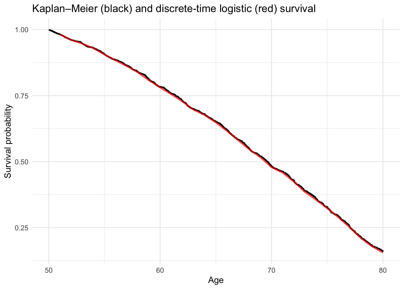

The curves essentially the same survival process, which illustrates an important point:

Kaplan–Meier and discrete-time logistic regression are not estimating completely different phenomena.

Both describe the same underlying process.

Kaplan–Meier estimates survival directly. The logistic regression estimates the interval-specific hazard, after which we reconstruct survival by accumulating those hazards:

\hat h_t \quad\longrightarrow\quad \prod_{k \leq t}(1-\hat h_k) \quad\longrightarrow\quad \hat S(t).

So why use regression at all?

Because regression allows us to introduce explanatory variables.

Adding covariates

We now extend the model by adding sex and socioeconomic status.

Code

m1 <- glm(
  death ~ factor(age) + sex + ses,
  data = scania_pp,
  family = binomial(link = "logit")
)

summary(m1)


Call:
glm(formula = death ~ factor(age) + sex + ses, family = binomial(link = "logit"), 
    data = scania_pp)

Coefficients:
              Estimate Std. Error z value Pr(>|z|)    
(Intercept)   -4.01420    0.18806 -21.345  < 2e-16 ***
factor(age)51  0.19612    0.24029   0.816 0.414388    
factor(age)52 -0.20922    0.27034  -0.774 0.438980    
factor(age)53  0.02659    0.25683   0.104 0.917529    
factor(age)54  0.37214    0.23908   1.557 0.119571    
factor(age)55  0.34943    0.24359   1.435 0.151423    
factor(age)56  0.30984    0.24879   1.245 0.212985    
factor(age)57  0.44695    0.24374   1.834 0.066695 .  
factor(age)58  0.73578    0.23218   3.169 0.001529 ** 
factor(age)59  0.64587    0.23952   2.696 0.007008 ** 
factor(age)60  0.61971    0.24404   2.539 0.011106 *  
factor(age)61  0.73214    0.24115   3.036 0.002397 ** 
factor(age)62  0.91162    0.23484   3.882 0.000104 ***
factor(age)63  0.49014    0.26264   1.866 0.062010 .  
factor(age)64  0.86770    0.24298   3.571 0.000355 ***
factor(age)65  1.06187    0.23643   4.491 7.08e-06 ***
factor(age)66  1.20193    0.23325   5.153 2.56e-07 ***
factor(age)67  1.25633    0.23456   5.356 8.50e-08 ***
factor(age)68  1.15485    0.24377   4.737 2.16e-06 ***
factor(age)69  1.48082    0.23305   6.354 2.10e-10 ***
factor(age)70  0.90005    0.27270   3.300 0.000965 ***
factor(age)71  1.48711    0.24195   6.146 7.93e-10 ***
factor(age)72  1.73238    0.23643   7.327 2.35e-13 ***
factor(age)73  1.51364    0.25430   5.952 2.64e-09 ***
factor(age)74  1.70035    0.25135   6.765 1.33e-11 ***
factor(age)75  1.87393    0.25057   7.479 7.51e-14 ***
factor(age)76  2.10797    0.24715   8.529  < 2e-16 ***
factor(age)77  2.36268    0.24628   9.594  < 2e-16 ***
factor(age)78  2.25939    0.26450   8.542  < 2e-16 ***
factor(age)79  2.16426    0.28492   7.596 3.05e-14 ***
sexfemale      0.04293    0.06283   0.683 0.494487    
seslower      -0.02372    0.07754  -0.306 0.759710    
---
Signif. codes:  0 '***' 0.001 '**' 0.01 '*' 0.05 '.' 0.1 ' ' 1

(Dispersion parameter for binomial family taken to be 1)

    Null deviance: 9121.7  on 27177  degrees of freedom
Residual deviance: 8684.7  on 27146  degrees of freedom
AIC: 8748.7

Number of Fisher Scoring iterations: 6

Age still represents the baseline hazard.

But the model now also allows mortality to differ according to:

sex;
socioeconomic status.

For example, the coefficient for sex describes how the log odds of dying during an interval differ between men and women at the same age and holding SES constant.

We could convert coefficients into odds ratios:

Code

exp(coef(m1))

  (Intercept) factor(age)51 factor(age)52 factor(age)53 factor(age)54 
   0.01805746    1.21667336    0.81121756    1.02695041    1.45083829 
factor(age)55 factor(age)56 factor(age)57 factor(age)58 factor(age)59 
   1.41825989    1.36320329    1.56353171    2.08710355    1.90764438 
factor(age)60 factor(age)61 factor(age)62 factor(age)63 factor(age)64 
   1.85838323    2.07953296    2.48836048    1.63253817    2.38141646 
factor(age)65 factor(age)66 factor(age)67 factor(age)68 factor(age)69 
   2.89176512    3.32652277    3.51249759    3.17353191    4.39656138 
factor(age)70 factor(age)71 factor(age)72 factor(age)73 factor(age)74 
   2.45973772    4.42427640    5.65408255    4.54323253    5.47583918 
factor(age)75 factor(age)76 factor(age)77 factor(age)78 factor(age)79 
   6.51381758    8.23153443   10.61935091    9.57721917    8.70817166 
    sexfemale      seslower 
   1.04386295    0.97656174

However, predicted probabilities and survival curves are generally easier to interpret.

Why adjusted survival curves?

Suppose men and women differ in their socioeconomic composition.

An ordinary Kaplan–Meier comparison between men and women reflects both:

differences associated with sex itself;
differences in the distribution of SES between the two groups.

Regression allows us to ask a different question:

What would predicted survival look like for men and women after accounting for differences in SES?

We can answer this using model-based standardization.

Rather than choosing one arbitrary SES category, we retain the observed SES distribution and predict survival under two counterfactual scenarios:

everyone is treated as male;
everyone is treated as female.

Everything else remains as observed.

Creating counterfactual prediction data

First create one baseline observation per person:

Code

baseline <- scania_pp |>
  distinct(
    id,
    sex,
    ses
  )

Now create every combination of:

person;
age;
hypothetical sex.

Code

prediction_data <- baseline |>
  select(id, ses) |>
  crossing(
    age = sort(unique(scania_pp$age)),
    sex_scenario = levels(scania_pp$sex)
  ) |>
  mutate(
    sex = factor(
      sex_scenario,
      levels = levels(scania_pp$sex)
    )
  )

Each person now appears at every age under both sex scenarios.

Their observed SES is retained.

This is important because we want to compare sex while averaging over the same SES distribution.

Predicting adjusted hazards with `marginaleffects`

Generate predicted interval-specific hazards:

Code

adjusted_hazards <- predictions(
  m1,
  newdata = prediction_data,
  type = "response"
) |>
  as.data.frame()

We now have a predicted probability of death for:

every individual;
every age;
each hypothetical sex.

For example:

Code

adjusted_hazards |>
  select(
    id,
    age,
    sex_scenario,
    ses,
    estimate
  ) |>
  head()

  id age sex_scenario   ses   estimate
1  1  50       female lower 0.01807499
2  1  50         male lower 0.01732865
3  1  51       female lower 0.02190557
4  1  51         male lower 0.02100444
5  1  52       female lower 0.01471296
6  1  52         male lower 0.01410344

The estimate column is again the discrete-time hazard.

From adjusted hazards to adjusted survival

For each hypothetical person, convert their sequence of hazards into survival:

Code

adjusted_survival_individual <- adjusted_hazards |>
  arrange(
    sex_scenario,
    id,
    age
  ) |>
  group_by(
    sex_scenario,
    id
  ) |>
  mutate(
    survival = cumprod(1 - estimate),
    age_end = age + 1
  ) |>
  ungroup()

We now have one predicted survival trajectory for every individual under each sex scenario.

To obtain the standardized survival curve, average these predicted survival probabilities across individuals:

Code

adjusted_survival <- adjusted_survival_individual |>
  group_by(
    sex_scenario,
    age_end
  ) |>
  summarise(
    survival = mean(survival),
    .groups = "drop"
  )

Plot the resulting curves:

Code

ggplot(
  adjusted_survival,
  aes(
    x = age_end,
    y = survival,
    linetype = sex_scenario
  )
) +
  geom_line(linewidth = 1) +
  labs(
    x = "Age",
    y = "Adjusted survival probability",
    linetype = "Sex",
    title = "SES-adjusted survival curves"
  ) +
  theme_minimal()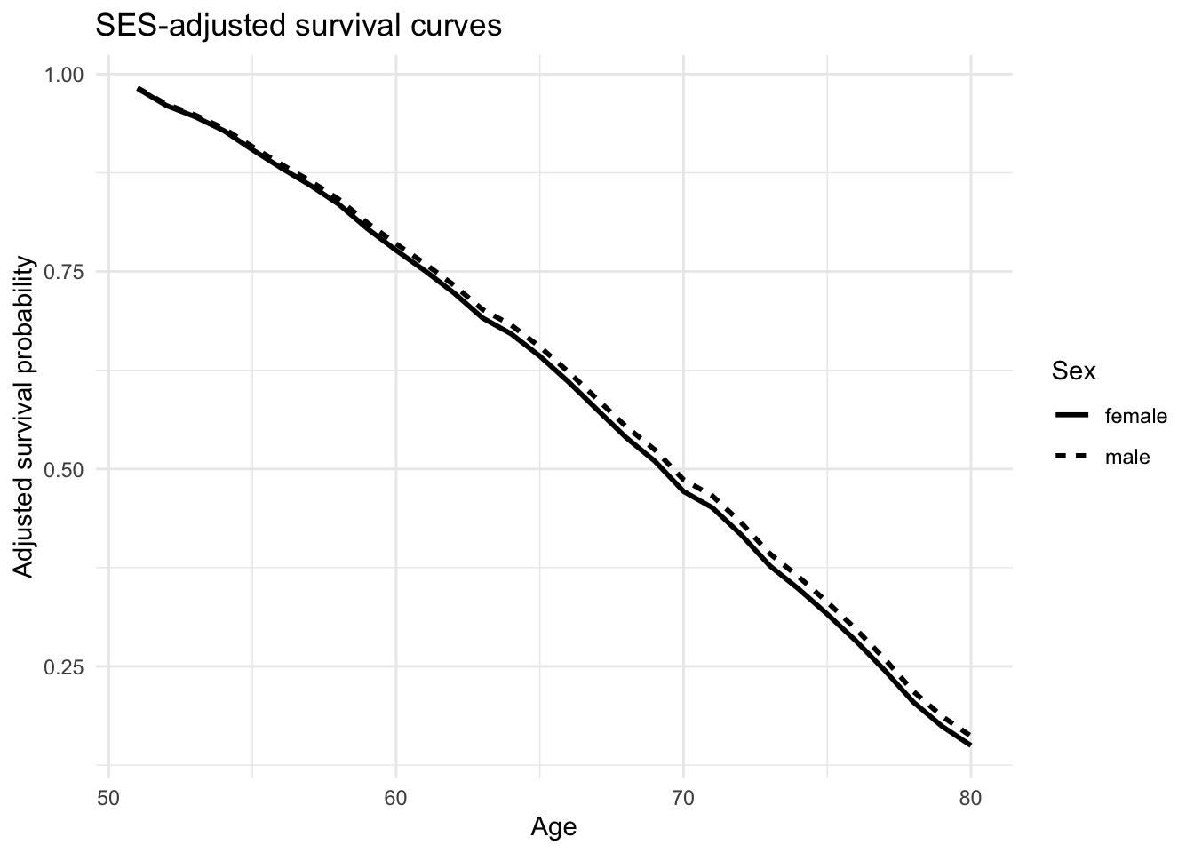

These curves can be interpreted as:

The predicted survival curves for men and women if both groups had the same SES distribution as the population in the data.

Unadjusted versus adjusted group differences

We can also look at the observed Kaplan–Meier curves separately by sex:

Code

km_sex <- survfit(
  Surv(enter, exit, event) ~ sex,
  data = scania
)

plot(
  km_sex,
  xlab = "Age",
  ylab = "Survival probability",
  lty = 1:2
)

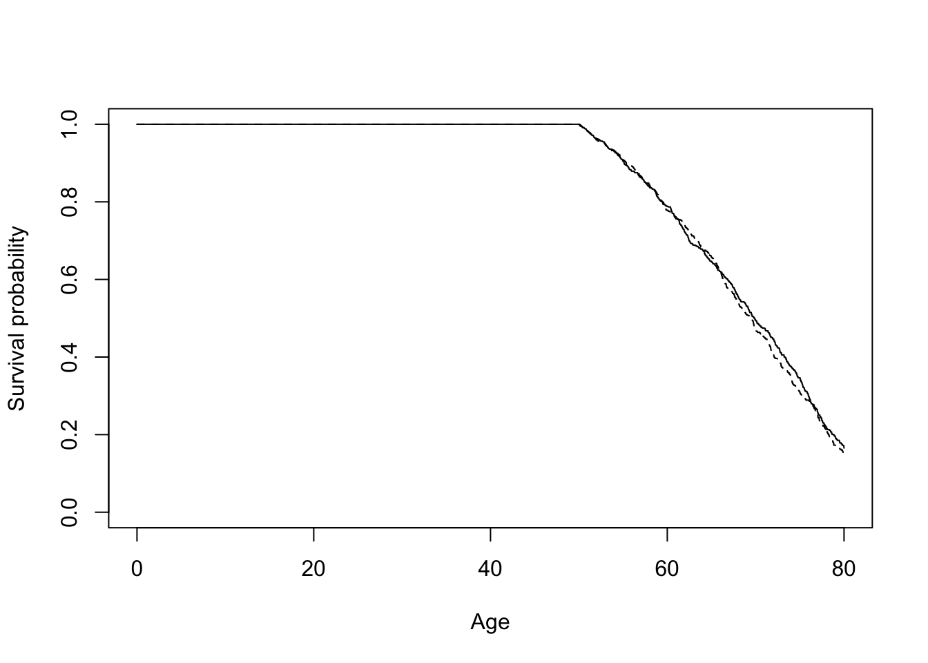
These are unadjusted survival curves.

They describe the actual survival experience of men and women in the data.

By contrast, the regression-based curves from the previous section are adjusted for SES.

Conceptually:

Kaplan–Meier by sex
        ↓
Observed / unadjusted difference

Regression + standardization
        ↓
Model-based difference after adjusting for SES

This distinction is one of the main reasons to move from Kaplan–Meier estimation to regression.

Comparing probabilities directly with `marginaleffects`

The regression model can also be used to compare predicted hazards directly.

For example:

Code

avg_comparisons(
  m1,
  variables = "sex",
  type = "response"
)


 Estimate Std. Error     z Pr(>|z|)   S    2.5 %  97.5 %
  0.00161    0.00236 0.683    0.495 1.0 -0.00302 0.00624

Term: sex
Type: response
Comparison: female - male

This converts the sex coefficient into an average difference in the predicted probability of death during an interval.

For instance, an estimate of

0.00161

would correspond to roughly a 0.2 percentage-point difference in the interval-specific probability of death, averaged across the observations used in the calculation.

This is often easier to interpret than an odds ratio.

Differences at particular ages

Because logistic regression is nonlinear, the same coefficient can correspond to different probability differences at different ages.

We can therefore estimate contrasts at specific ages:

Code

comparisons(
  m1,
  variables = "sex",
  newdata = datagrid(
    age = c(60, 70, 79),
    ses = unique
  ),
  type = "response"
)


 age   ses Estimate Std. Error     z Pr(>|z|)   S    2.5 %  97.5 %
  60 upper  0.00138    0.00203 0.676    0.499 1.0 -0.00261 0.00536
  60 lower  0.00135    0.00198 0.680    0.497 1.0 -0.00253 0.00523
  70 upper  0.00178    0.00264 0.675    0.500 1.0 -0.00340 0.00696
  70 lower  0.00174    0.00257 0.678    0.498 1.0 -0.00330 0.00679
  79 upper  0.00512    0.00757 0.676    0.499 1.0 -0.00971 0.01995
  79 lower  0.00503    0.00741 0.679    0.497 1.0 -0.00949 0.01956

Term: sex
Type: response
Comparison: female - male

The general principle is:

Do not assume that a constant logit coefficient implies a constant difference in probabilities.

Modeling the baseline hazard differently

For the first model we used:

factor(age)

This is useful because it imposes essentially no functional form on the age pattern of mortality.

But it requires many parameters.

Once the basic logic is clear, we could use a smoother specification.

For example, a quadratic:

Code

m_quad <- glm(
  death ~ age + I(age^2) + sex + ses,
  data = scania_pp,
  family = binomial(link = "logit")
)

Or, usually more flexibly, a spline:

Code

m_spline <- glm(
  death ~ splines::ns(age, df = 4) + sex + ses,
  data = scania_pp,
  family = binomial(link = "logit")
)

The difference is that these models impose some smoothness on the baseline hazard.

Logit versus complementary log-log

So far we have used:

family = binomial(link = "logit")

This gives a discrete-time logistic event history model.

Another common specification is:

family = binomial(link = "cloglog")

For example:

Code

m_cloglog <- glm(
  death ~ factor(age) + sex + ses,
  data = scania_pp,
  family = binomial(link = "cloglog")
)

The complementary log-log model has a particularly close connection to continuous-time proportional hazards models.

For short intervals and relatively uncommon events, logit and complementary log-log models often produce similar predicted hazards.

The logic of the analysis

The whole exercise can now be understood as one sequence:

\text{survival data} \rightarrow \text{Kaplan–Meier}

followed by

\text{person-period data} \rightarrow \text{logistic model of the hazard} \rightarrow \hat h_t \rightarrow \prod_t (1-\hat h_t) \rightarrow \hat S(t).

With no covariates, this gives us another way to describe the same basic survival process estimated by Kaplan–Meier.

Once covariates are introduced, the regression model allows us to move beyond description and calculate survival curves under different covariate scenarios.

The key insight is therefore not simply that logistic regression can be used for EHA.

It is that a discrete-time survival process can be decomposed into a sequence of conditional binary probabilities:

P(event_t=1 \mid event_{t-1}=0).

Model those probabilities, and we model the hazard.

Accumulate them, and we recover survival.

Reuse

CC BY 4.0

Citation

BibTeX citation:

@online{fang2026,
  author = {Fang, Christian},
  title = {Event {History} {Analysis} in {R}},
  date = {2026-10-18},
  url = {https://www.christianfang.eu/posts/eha/},
  langid = {en}
}

For attribution, please cite this work as:

Fang, Christian. 2026. “Event History Analysis in R.” October 18, 2026. https://www.christianfang.eu/posts/eha/.

Introduction

Setup

Survival and the hazard

Kaplan–Meier survival

Person-Period files

Discrete-time EHA using logistic regression

First model: the baseline hazard only

Predicted hazards using marginaleffects

From predicted hazards back to survival

Comparing logistic regression with Kaplan–Meier

Adding covariates

Why adjusted survival curves?

Creating counterfactual prediction data

Predicting adjusted hazards with marginaleffects

From adjusted hazards to adjusted survival

Unadjusted versus adjusted group differences

Comparing probabilities directly with marginaleffects

Differences at particular ages

Modeling the baseline hazard differently

Logit versus complementary log-log

The logic of the analysis

Reuse

Citation

Predicted hazards using `marginaleffects`

Predicting adjusted hazards with `marginaleffects`

Comparing probabilities directly with `marginaleffects`